Protein dynamics and disorder

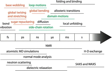
Although we often visualise proteins in terms of a static structure, all proteins undergo motions on a wide range of timescales, many of which are functionally important. NMR provides tools for measuring these dynamics in both folded and intrinsically disordered proteins. A number of applications are discussed below.

Examples of different timescales of dynamics in biomolecules. Bond vibration occurs on the fs timescale; sidechain rotation can take ps to ms; loop motions typically occur on the ns to us timescale; domain motions can take from ns to ms; folding, binding and allosteric transitions can take from us to s. — Some examples of dynamic processes in biomolecules and their timescales. Based on figure 2 in Fenwick, Esteban-Martin, Salvatella (2011) *European Biophysics Journal* 40 1339-1355 DOI: https://doi.org/10.1007/s00249-011-0754-8

Backbone flexibility

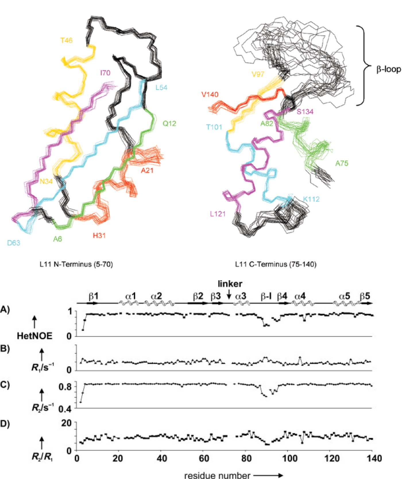
There are several NMR methods that give information on backbone flexibility. As discussed in the pages on 1D experiments and ¹⁵N-HSQCs, you can tell if a protein is globally disorded by looking at the distribution of chemical shifts. To get more detail on specific residues, you can record variants of the ¹⁵N-HSQC experiment that record the relaxation properties of amide ¹⁵N nuclei along the backbone. These relaxation properties can be combined to estimate the timescale and amplitude of motions along the backbone, using model-free analysis and software such as Relax.

A complement/alternative to ¹⁵N relaxation studies is to predict the backbone flexibility from the carbon chemical shifts measured during the backbone assignment process. Secondary structure causes characteristic changes in the carbon chemical shifts, while flexibility tends to move them towards average "random coil" values. Programs such as TALOS-N can use these shifts to estimate the S2 order parameter, which is correlated to the amplitude of motions along the backbone.

Above, NMR ensembles of L11 ribosomal protein N and C terminal domains, showing flexibility of some loops. Below, 15N relaxation measurements which confirm the beta loop in the C domain is flexible. — The upper part shows the N- and C-terminal domains of the ribosomal protein L11 from *Thermotoga maritima*, as solved by NMR. The ensemble shows a lot more variation in the C-terminal domain, especially around the beta loop. Below is 15N relaxation data that confirm that beta loop is especially flexible. This region is functionally important, as it is involved in binding to the ribosomal RNA. Based on figure 4 in Ilin et al (2005) *ChemBioChem* 6 1611-1618 DOI: https://doi.org/10.1002/cbic.200500091. See also the Schwalbe group website.

Transitions between conformations/oligomeric states

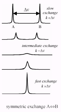
Some processes cause larger changes to the entire protein or to a subregion: these include global changes in conformation (eg transitioning between open and closed forms) or formation of oligomers or complexes. These transitions usually result in change in peak position and/or intensity in the ¹⁵N-HSQC. The exact appearance depends on the rate at which the protein transitions between the states: for processes which are fast on the NMR timescale (typically k_ex > 100-1000 /s), the peak will move to the weighted average of the two states; while for slow processes (k_ex < 10-100 /s), seperate peaks may be observed for the two states, and information on exchange rates extracted using EXSY experiments. (There is unfortunately an intermediate regime where signals tend to disappear entirely, showing that an exchange process is occurring but not revealing its details - this typically happens when k_ex is roughly 100-1000 /s).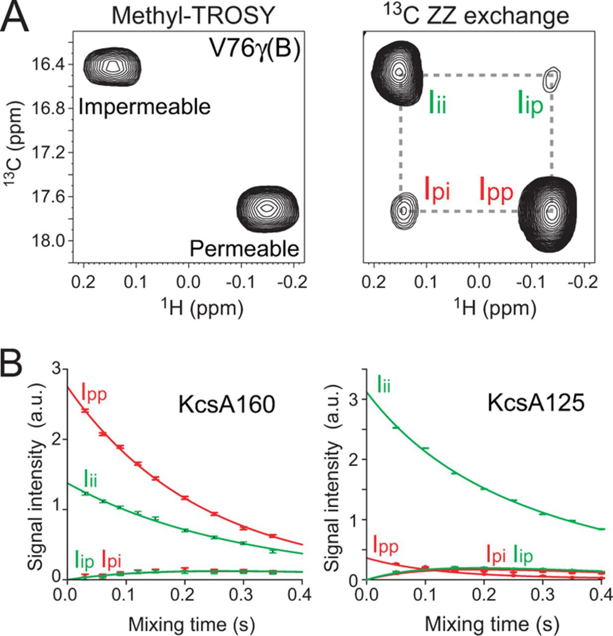

Above left, a section of a 13C TROSY spectrum showing peaks for permeable and impermeable states; above right, an EXSY spectrum which shows cross peaks between the two states. Below, plots of EXSY peak intensity against mixing time. — The upper left panel shows peaks corresponding to permeable and impermeable states of the K⁺ channel KcsA from *Streptomyces lividans*. The appearance of two distinct peaks shows that these states are in slow exchange. The upper right panel shows an EXSY experiment (aka ZZ exchange) which demonstrates some exchange between states after a fixed mixing. By repeating this experiment with different mixing times, you can create plots like those in the bottom half of the figure - fitting this data gives the exchange rate. Reproduction of figure 3 in Imae et al (2012) *Journal of Biological Chemistry* 287 39634-39641 DOI: https://doi.org/10.1074/jbc.M112.401265.

Note on timescales in NMR

We can categorise dynamic processes as fast, intermediate or slow with respect to the NMR timescale, but what do we mean by this? As an example, consider two protein states that can exchange, and focus on one atom that is different between them. Because this atom is in a different chemical environment in the two states, it will have different chemical shifts. Although we usually measure chemical shifts in ppm compared to a reference, they really represent the precession frequency of the nuclear spin, and can be measured in Hz.

The appearance of the NMR spectra depends on how the frequency difference between the states compares to the rate of exchange between them. If the exchange rate is much slower, you observe two separate peaks in the spectrum. On the other hand, if the exchange rate is faster than the frequency difference then you observe a single sharp peak at the average frequency. When the exchange rate is similar to the frequency difference, a single broad peak is seen.

To give a concrete example, suppose we are looking at a proton which differs in chemical shift by 1 ppm between the two states: on our instrument, that corresponds to a frequency difference of 700 Hz, or a timescale or 1-2 ms. Exchange processes that are much faster than this (such as exchange between conformers in an intrinsically disordered protein) will give rise to a single peak, while exchange processes that are much slower (such as dissociation of a tightly bound ligand) will give rise to two separate peaks.

Series of NMR spectra with different exchange rates. Two sharp peaks are seen for fast exchange, a single broad peak for intermediate exchange, and a single sharp peak for fast exchange — Appearance of 1D NMR spectra with exchange at different timescales. Image from http://triton.iqfr.csic.es/guide/eNMR/restraints/exchange.html

Transitions to rare/excited conformations

Sometimes the interesting state of a protein isn't the most populated state, but is instead a transient, excited state. This can be the case for multi-step enzyme reactions, or for proteins which are regulated by a switch between active and inactive states. These transient states are typically too low in concentration to be observed directly, but several NMR techniques can indirectly detect and characterise them through observation of the more populated state. These techniques include Chemical Exchange Saturation Transfer (CEST) and relaxation dispersion, and are suitable even for systems in intermediate exchange.

Side chain dynamics

¹³C nuclei can be used as probes of side chain dynamics in the same way that ¹⁵N nuclei are used to probe the dynamics of the backbone. Similar experiments can be used: relaxation measurements to probe fast motions, and chemical exchange and relaxation dispersion to probe slower motions. These methods are particularly applicable to methyl groups or aromatic side chains. The main caveat is that the side chains must typically be isotopically labelled only at specific sites (to avoid interference from J coupling between neighbouring carbons), which requires the use of expensive specifically-labelled amino acids in the growth medium.

Requirements

Most of the dynamics experiments above require ¹⁵N labelled protein at a reasonably high concentration (at least 200 uM, but preferably higher). ¹³C labelling is not necessary in most cases, although may be needed for more specialised experiments, or ones which look at side chain dynamics.